How to read and build a mortality table

Photo by Miguel Bruna on Unsplash

Mortality tables serve as a foundation for computing vital metrics like life expectancy and the median age of death. Proficiency in utilising mortality tables holds significant value across diverse business sectors. Data scientists working in financial planning, risk assessment, and insurance-related endeavors can leverage this knowledge to determine life insurance premiums and pension contributions and model the risk and exposure of the firm. Additionally, these tables can inform marketing strategies when age distribution and mortality rates allow to model the revenue potential for a given population, for instance for the creation of a new drug in the pharmaceutical industry. The concepts extend to other domains like subscription services, where churn analysis extracts knowledge from tables showcasing subscriber attrition rates and where basic metrics like ARPU and LTV are easy to communicate to management. This approach can be adapted to asset management within a company, for the modeling of asset lifecycles and depreciation, among other applications.

So let’s start with an easy example to see what are the main metrics you should be looking at when dealing with such a table. After that, we’ll look at a real mortality table from the ONS in the UK.

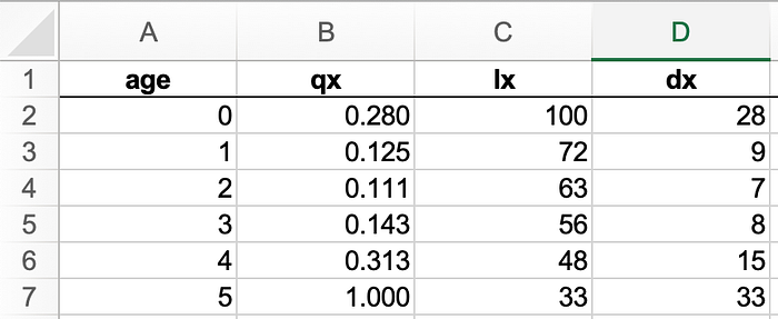
To make things easy, let’s start with a very simple example: a population of 100 people who all die within 6 years (from year 0 to the end of year 5):

The age variable x represents the age interval x to x+1

lx represents the number of people surviving until age x,

dx the number of people dying between age x and x+1

And qx is the mortality rate, i.e. the proportion of people dying between age x and x+1 so qx=dx/lx

How can we calculate the life expectancy from those numbers? There are two equivalent ways to interpret at life expectancy: the average (mean) number of years lived in a given population or the average (mean) age of death.

Let’s consider the first definition, to calculate it we need to add a new variable to the table, usually called Lx, the total person-years lived above age x or the total number of years lived in the population for people between the age of x and x+1. Let’s take an example: at age 2, we can see from the table that we have 63 people reaching that age (l2=63) and only 56 surviving to age 3 (l3=56). So that’s 56 people living one full year each plus 7 living less than one year (we usually take 6 months as an average) so that gives L2=56+3.5=59.5. As a side note, this is the same as calculating (lx+1 + lx)/2. So for example, the formula in Excel for age 3, would be: =C6+D5/2
From Lx we can derive Tx, the total number of years lived (Tx) from age x till the end, so simply the sum of all the Lx from age x till age 5 in our table (the last option)

We can now update our table with those 2 new columns:

Can you see how Tx is derived from Lx?

The last step is to take Tx, and divide it by the number of people at the start of each period, lx. We do that at every age, to get the life expectancy at age x (denoted ex). This gives us the following table:

Now we can also look at it from the other point of view: life expectancy as the average age at which people die. In that case we take a weighted average of the age of death (taking the midpoint for each age), so for instance in this case: 28 people die between age 0 and 1 (so we take 6 months), 9 die at age 1.5, 7 at 2.5 etc. we simply take the average and get exactly the same values.

Now moving to the next concept, the median age of death. The median age of death is simply the age at which half of the population has passed away, so from the table, what age would that be? If you said “at some point between the age of 3 and 4”, you’d be right, this is when only 50 people are still alive and is somewhat close to our mean life expectancy at birth of 3.2.

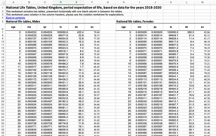
That should be pretty straightforward, so let’s use some real data from the Office for National Statistics in the UK (https://www.ons.gov.uk/peoplepopulationandcommunity/birthsdeathsandmarriages/lifeexpectancies/datasets/nationallifetablesunitedkingdomreferencetables).

Screenshot of the tables from the ONS website

As you can see, the tables are separated by gender and you should by now be in a position to calculate all those numbers if you only had the values for the mortality rate qx. Note that there is an additional variable present in the table, mx, defined by the ONS as “the central rate of mortality, defined as the number of deaths at age x last birthday in the three year period to which the National Life Table relates divided by the average population at that age over the same period.” So for example mx for age 60 in 2018 to 2020 would be the average number of deaths at age 60 across 2018, 2019 and 2020, divided by the average number of people aged 60 across 2018, 2019 and 2020. This value is generally used to calculate qx.

We also need to slightly tweak the calculation of the life expectancy to take into account two factors:

i. infant birth happens with different patterns and so taking the midpoint (6 months) is not good enough.

ii. The last age in the table should really read “100 and over” and so we need to account for the fact that there are people living longer than 100 years.

There are several methods to correct for (i) and the values are usually calculated from real data. In the absence of data, here is what the World Health Organisation (WHO) recommends using:

How to correct for infant mortality, WHO guidelines

For (ii), 4 main methods can be used:

• The Forced Method: assume a mortality rate at the last age to 1.
• The Blended Method: blend the rates from some earlier age to decrease smoothly into 1 at the last age.
• The Pattern Method: let the pattern of mortality continue until the rate gets to 1 and use that as the ultimate age.
• The Less-Than-One Method: select an ultimate age but end the table at whatever rate is produced at that age so that the ultimate rate is less than 1

You can read more on the subject on the website of the Society of Actuaries (SOA) here: https://www.soa.org/globalassets/assets/files/resources/essays-monographs/2005-living-to-100/m-li05-1-ix.pdf

To end this short introduction, let’s use Python to calculate those rates and a few additional metrics

import pandas as pd
data = pd.read_csv('uk-mortality.csv')
data=data[['age','lx']]
data

This is our table, with only the age and the people surviving for each age bracket:

# We can easily calculate the number of deaths dx for each age group
data['dx']=(data['lx'].shift(1)-data['lx']).shift(-1)
data.loc[100,('dx')]=data.loc[100,'lx']
# Let's add qx, the probability of dying between age x and age x+1
data['qx'] = data['dx']/data['lx']
# And px, the probability of surviving from age x until age x+1
data['px'] = 1-data['qx']
data

Let’s now add a few new concepts (you can get more info on the Actuaries.org.uk website)

tPx: tpx represents the probability that a person aged exactly x lives for another t years to exact age (x+t): tpx = l(x+t) / lx

tqx: tqx represents the probability that a person aged exactly x dies before exact age (x+t): tqx = 1 — tpx

# The probability of someone who is turning 18 now living until 60
data['lx'][60]/data['lx'][18]

0.9117419744389655

# The probability of someone who's turning 18 now dying before turning 60
(data["lx"][18]-data["lx"][60])/data["lx"][18]

0.08825802556103449

m|nqx: m|nqx is the probability that a person aged exactly x dies between exact ages (x+n) and (x+m+n): m|nqx = ( l(x+n) — l(x+m+n) ) / lx

Let’s find the probability of a person aged exactly 18 dying between ages 60 and 80, that is, 20|42q18

(data["lx"][60]-data["lx"][80])/data["lx"][18]

0.33090671228741075

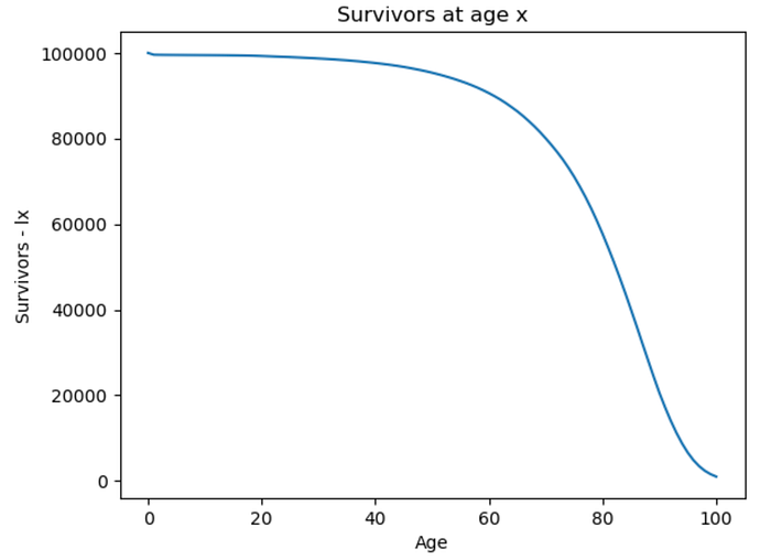
Finally, we’ll cover the last concept, force of mortality, µx, representing the instantaneous rate at which people are dying. There is a very good explanation here: https://www.youtube.com/watch?v=AitvcGqPeJM but essentially we could imagine that the number of survivors is a continuous function, that can be viewed if we plot lx:

import matplotlib.pyplot as plt

plt.plot(data.age, data.lx)
plt.xlabel('Age')
plt.ylabel('Survivors - lx')
plt.title('Survivors at age x')
plt.show()

We can see from our mortality table that the probability of dying between age 1 and 2 is 0.000231 but between age 2 and 3 it is 0.000131 so we could wonder what that probability would be at exactly 1 year and 4 months, for example…intuitively we know the value should be somewhere between those 0.000231 and 0.000131. We also know that the probability of death is not constant across ages:

plt.plot(data.age, data.qx)
plt.xlabel('Age')
plt.ylabel('qx - probability of death')
plt.title('Probability of death')
plt.show()

So if we can approximate those curves using a continuous function, we can calculate the derivative at any point to get the instantaneous rate of death, µx. The British mathematicians Benjamin Gompertz and William Makeham designed a way to approximate those tables with a continuous function, including an exponential increase in death rates with age (more about it here).

Here, we’ll simply use an approximation:

𝜇𝑥 ≈ −.5 * (log(𝑝𝑥−1)+log(𝑝𝑥))

import numpy as np
data["μx"]=0.0
for x in range(1,101):
     data.loc["μx",x] = -.5*(np.log(data["px"][x-1]) + np.log(data["px"][x]))

That’s it for that short introduction, basically we have seen how to calculate total life expectancy at different ages, the probability of dying between two specific ages, the notion of force of mortality and got an intuition for what the median life expectancy is.